Sampling from a different Gaussian

One way to evaluate integral ratios of the form $\langle f \rangle_\varrho = \frac{ \int\! \mathrm{d} x \, \varrho(x) f(x) }{ \int\! \mathrm{d} x \, \varrho(x) }$ is using Monte Carlo integration. If $\varrho(x)$ is proportional to the pdf of a Gaussian distribution, $\varrho(x) \propto \exp\left( -\frac{(x - \mu)^2}{2 \sigma^2} \right),$ then sampling is very easy, with many languages and environments offering a function for rejection-free sampling (e.g. Julia's randn).

For example, we choose the function $f(x) = x^2$ and a Gaussian distribution $\varrho(x)$ with mean $\mu = 2.5$ and standard deviation $\sigma = 1.5$. From the definition of the variance ($\sigma^2 = \langle x^2 \rangle - \mu^2$), we see that $\langle f \rangle_\varrho = \mu^2 + \sigma^2 = 8.5.$ If we perform the average $\bar{f} = \frac{1}{N} \sum_{i=1}^N f(x_i)$ for $N = 10^4$ samples and bin the results over many trials, the distribution looks like

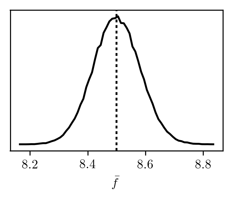
Single Gaussian

Suppose that we want to evaluate the same integral ratio as before, but by sampling from a different Gaussian distribution $\varrho'(x')$ with mean $\mu' = -1.2$ and standard deviation $\sigma' = 2.8$. We introduce $x'(x) = \frac{\sigma'}{\sigma} (x - \mu) + \mu',$ so that $\varrho(x) \propto \varrho'(x'(x)).$ This gives us $\langle f \rangle_\varrho = \frac{ \int\! \mathrm{d} x \, \varrho'(x'(x)) f(x) }{ \int\! \mathrm{d} x \, \varrho'(x'(x)) },$ to which we apply a change of variables from $x$ to $x'$, yielding $\langle f \rangle_\varrho = \frac{ \int\! \mathrm{d} x' \, \varrho'(x') f'(x') }{ \int\! \mathrm{d} x' \, \varrho'(x') },$ where $f'(x') = f(x(x')) = f\left( \frac{\sigma}{\sigma'} (x' - \mu') + \mu \right).$ We don't need to worry about $\frac{\mathrm{d} x}{\mathrm{d} x'} = \frac{\sigma}{\sigma'},$ because it would appear in both the numerator and denominator.

Hence, we see that $\langle f \rangle_\varrho = \langle f' \rangle_{\varrho'}.$ We may verify that this is the case by sampling from $\varrho'$ and evaluating $\bar{f}' = \frac{1}{N} \sum_{i=1}^N f\left( \frac{\sigma}{\sigma'} (x_i' - \mu') + \mu \right).$ Binning the results from several trials, we obtain 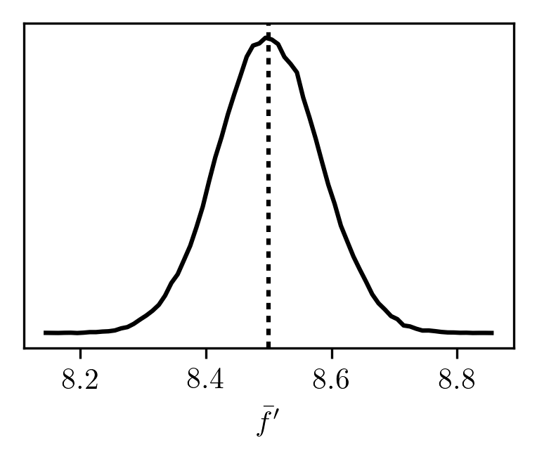As expected, this distribution looks very similar to the previous one.

From an implementation perspective, this result is incredibly trivial. Since in practice we obtain random values from a standard Gaussian distribution (with zero mean and unit variance), sampling from a Gaussian with specific parameters amounts to a scaling and a shift:

1

xs1 = 1.5 * randn(SAMPLE_SIZE) + 2.5

It is then clear that sampling with any other parameters and performing the described transformation is functionally identical:

1
2

xs2 = 2.8 * randn(SAMPLE_SIZE) + (-1.2)
xs1 = (xs2 - (-1.2)) * 1.5 / 2.8 + 2.5

Multiple Gaussians

The case of several independent Gaussians is a straightforward generalization of the above. In principle, multiple correlated Gaussians may always be transformed into independent Gaussians, so we may stop here. However, it is interesting to see what the transformation for the sampled values is in terms of the original coordinates.

We now consider a distribution $\varrho$ with mean vector $\vec{\mu}$ and covariance matrix $\mathbf{\Sigma}$, whose pdf is $\varrho(\vec{x}) \propto \exp\left( -\frac{1}{2} (\vec{x} - \vec{\mu})^\mathrm{T} \mathbf{\Sigma}^{-1} (\vec{x} - \vec{\mu}) \right).$ For convenience, we introduce $\mathbf{A} = \mathbf{\Sigma}^{-1}$ and diagonalize it as $\mathbf{A} = \mathbf{S}^\mathrm{T} \mathbf{\Lambda} \mathbf{S}$. If we have another distribution $\varrho'$ with parameters $\vec{\mu}'$ and $\mathbf{\Sigma}'$, then the choice $\vec{x}'(\vec{x}) = (\mathbf{S}')^\mathrm{T} \sqrt{(\mathbf{\Lambda}')^{-1} \mathbf{\Lambda}} \mathbf{S} (\vec{x} - \vec{\mu}) + \vec{\mu}'$ results in $\varrho(\vec{x}) \propto \varrho'(\vec{x}'(\vec{x})).$ This is essentially identical to the univariate $x'(x)$, but with the introduction of the transformation matrices $\mathbf{S}$ and $\mathbf{S}'$ to decouple the coordinates.

As before, we have that $\langle f \rangle_\varrho = \langle f' \rangle_{\varrho'},$ where $f'(\vec{x}') = f(\vec{x}(\vec{x}')) = f\left( \mathbf{S}^\mathrm{T} \sqrt{\mathbf{\Lambda}^{-1} \mathbf{\Lambda}'} \mathbf{S}' (\vec{x}' - \vec{\mu}') + \vec{\mu} \right).$ Again, this is not surprising if we consider what is done operationally when sampling from independent standard Gaussian distributions.

We may check this result with $\vec{\mu} = \begin{pmatrix} -0.6 & 1.4 \end{pmatrix},$ $\mathbf{\Sigma} = \begin{pmatrix} 2 & 1 \\ 1 & 3 \end{pmatrix},$ $\vec{\mu}' = \begin{pmatrix} 0.6 & -1.4 \end{pmatrix},$ $\mathbf{\Sigma}' = \begin{pmatrix} 3 & -1 \\ -1 & 2 \end{pmatrix},$ and $f(\vec{x}) = (x_1 + x_2)^2.$ The resulting distributions are: 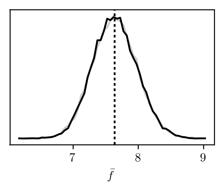The grey curve is from sampling $\varrho$, while the black curve is from sampling $\varrho'$ and then transforming the sampled coordinates. The exact result (dotted) is given by $(\mu_1 + \mu_2)^2 + \frac{(s_{11} + s_{12})^2}{\lambda_1} + \frac{(s_{21} + s_{22})^2}{\lambda_2} = 7.64.$ So far, we've seen that sampling from any Gaussian is as good as any other.

Application: Finite difference

Consider the function $F(p) = \langle f(p) \rangle_p = \frac{ \int\! \mathrm{d} x \, \varrho(p, x) f(p, x) }{ \int\! \mathrm{d} x \, \varrho(p, x) },$ where $x$ is a scalar or a vector. We may approximate its derivative using a finite difference formula: $\frac{\mathrm{d} F}{\mathrm{d} p} \approx \frac{1}{2 \Delta p} (F(p + \Delta p) - F(p - \Delta p)).$ More elaborately, its log derivative is given by $\frac{\mathrm{d} \ln{F}}{\mathrm{d} p} \approx \frac{1}{2 \Delta p} \cdot \frac{ F(p + \Delta p) - F(p - \Delta p) }{ F(p) }.$ This is equivalently written as $\frac{\mathrm{d} \ln{F}}{\mathrm{d} p} \approx \frac{1}{2 \Delta p} \cdot \frac{ \langle f(p + \Delta p) \rangle_{p + \Delta p} - \langle f(p - \Delta p) \rangle_{p - \Delta p} }{ \langle f(p) \rangle_p }.$

Suppose that sampling is the most expensive part of the calculation and so we only wish to sample values from a single distribution. From the above discussion, we know that there are functions $f^+(x)$ and $f^-(x)$ such that $\frac{\mathrm{d} \ln{F}}{\mathrm{d} p} \approx \frac{1}{2 \Delta p} \cdot \frac{ \langle f^+ \rangle_p - \langle f^- \rangle_p }{ \langle f(p) \rangle_p },$ where the only approximation is due to the finite difference. Specifically, $f^\pm(x) = f(p \pm \Delta p, x^\pm(x)),$ where $x^\pm(x)$ are the appropriate coordinate transformations. Hence, we may estimate this derivative by sampling from just one distribution rather than three.

For example, consider the multivariate Gaussian $\varrho(p, \vec{x})$ with $\vec{\mu} = \begin{pmatrix} -0.6 & 1.4 \end{pmatrix},$ and $\mathbf{\Sigma}(p) = \begin{pmatrix} 2 p & 1 \\ 1 & 3/p \end{pmatrix}.$ If we choose the function $f(p, \vec{x}) = p^2 (x_1 + x_2)^2,$ then $F(p=1) = 7.64$ is the value we were estimating in the previous section. Now we will estimate $\left. \frac{\mathrm{d} \ln{F}}{\mathrm{d} p} \right|_{p=1}$ with $\Delta p = 10^{-4}$. The distributions that we get are: 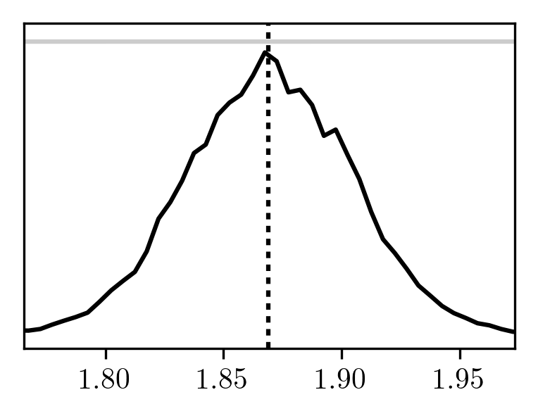The black curve is generated by sampling only from $\varrho(p, \vec{x})$ (and not $\varrho(p + \Delta p, \vec{x})$ or $\varrho(p - \Delta p, \vec{x})$). The dotted line is found by applying the finite difference method to the exact result. The grey curve (which looks like a horizontal line in the above plot) shows what happens if we sample from all three distributions separately. To really appreciate the difference between the two, it helps to zoom out:

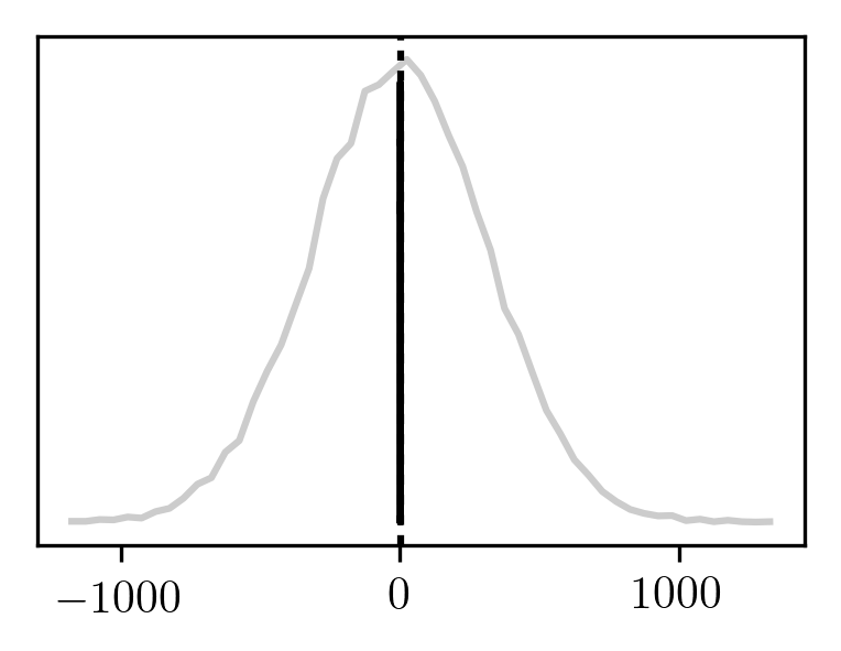
Surprisingly, it seems that we not only save on sampling effort using this technique, but we also significantly reduce the standard error of the mean! This reduction might be due to a favourable cancellation of errors that is only possible when the sampled points are the same.

We may also try to evaluate the derivative of a more convoluted expression. Starting from $F(p) = \frac{ \int\! \mathrm{d} x \, g(p, x) }{ \int\! \mathrm{d} x \, \varrho(p, x) },$ we may always obtain $F(p) = \langle f(p) \rangle_p = \frac{ \int\! \mathrm{d} x \, \varrho(p, x) f(p, x) }{ \int\! \mathrm{d} x \, \varrho(p, x) }$ by setting $f(p, x) = \frac{g(p, x)}{\varrho(p, x)}.$

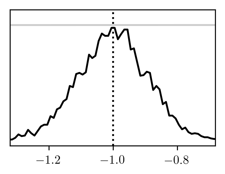
For our example, we'll use $g(p, \vec{x}) = \exp\left( -p (x_1^2 + x_2^2) \right)$ and the same $\varrho(p, \vec{x})$ as before. 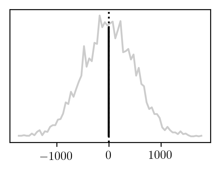We obtain a simple form for the expression: $F(p) \propto \frac{\sqrt{\lambda_1 \lambda_2}}{p}.$ Because $\lambda_1 \lambda_2$ is the determinant of $\mathbf{A}$, which happens to be constant, we have that $\frac{\mathrm{d} \ln{F}}{\mathrm{d} p} = -\frac{1}{p}.$ Sampling the finite difference at $p=1$ yields and Once again, we see an improvement if we only sample once.

It appears that although sampling from one Gaussian and then swapping it out for a different one is formally a useless procedure, there do exist situations where it provides some benefit.