Restricted Boltzmann machine parameters for a product distribution

2018-11-21

A restricted Boltzmann machine (RBM) is a tool for modelling discrete probability distributions. Specifically, it's a collection of numbers (weights $W_{ij}$ and biases $a_i$ , $b_j$ ), along with algorithms for training (setting the weights and biases to reflect the desired distribution) and sampling (obtaining samples that are distributed according to the desired distribution).

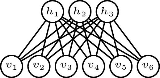
The joint probability distribution for an RBM is $P(v, h) \propto e^{a^\mathrm{T} v + b^\mathrm{T} h + v^\mathrm{T} W h}.$ Here, the vector $v$ (resp. $h$ ) represents the visible (resp. hidden) units, and each element $v_i$ (resp. $h_i$ ) can take on the values $0$ and $1$ . Pictorially, this looks like the following: Schematic of a general restricted Boltzmann machine. In this example, there are $N_v = 6$ visible units, $N_h = 3$ hidden units, and $N_v N_h = 18$ weights connecting them.

The hidden units are an artifact of the model; the actual distribution being modelled is only for the visible units $v$ . The effective distribution that we obtain from the RBM is the marginal distribution $P(v) = \sum_h P(v, h),$ where the sum over $h$ is understood to run over all $2^{N_h}$ states of the hidden layer. The question that I have in mind is the following: What are the appropriate weights and biases so that $P(v)$ is a product of univariate distributions over $v_i$ ?

We can express the marginal distribution as $\begin{aligned} P(v) &\propto \sum_h e^{a^\mathrm{T} v + b^\mathrm{T} h + v^\mathrm{T} W h} \\ &= e^{\sum_{i=1}^{N_v} a_i v_i} \sum_h e^{\sum_{j=1}^{N_h} (b^\mathrm{T} + v^\mathrm{T} W)_j h_j} \\ &= \left[ \prod_{i=1}^{N_v} e^{a_i v_i} \right] \left[ \prod_{j=1}^{N_h} \left( 1 + e^{b_j + (v^\mathrm{T} W)_j} \right) \right]. \end{aligned}$ The $v_i$ are in general coupled via the weights, so we will make a simplifying assumption: we require that the weight matrix $W$ have no more than one non-zero entry in each row and each column. Without loss of generality, we can place these entries on the diagonal and call them $W_i = W_{ii}$ , since that only amounts to rearranging the visible and hidden units. If $N_v < N_h$ , the weight matrix then has the form $\begin{pmatrix} W_1 & 0 & 0 & 0 & 0 & 0 & 0 \\ 0 & W_2 & 0 & 0 & 0 & 0 & 0 \\ 0 & 0 & W_3 & 0 & 0 & 0 & 0 \\ 0 & 0 & 0 & W_4 & 0 & 0 & 0 \end{pmatrix},$ if $N_v = N_h$ , it has the form $\begin{pmatrix} W_1 & 0 & 0 & 0 \\ 0 & W_2 & 0 & 0 \\ 0 & 0 & W_3 & 0 \\ 0 & 0 & 0 & W_4 \end{pmatrix},$ and if $N_v > N_h$ , it has the form $\begin{pmatrix} W_1 & 0 & 0 & 0 \\ 0 & W_2 & 0 & 0 \\ 0 & 0 & W_3 & 0 \\ 0 & 0 & 0 & W_4 \\ 0 & 0 & 0 & 0 \\ 0 & 0 & 0 & 0 \\ 0 & 0 & 0 & 0 \end{pmatrix}.$ Thus, under this assumption only the first $\min(N_v, N_h)$ visible and hidden units are allowed to be connected, and only pairwise. 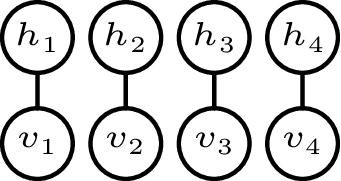For brevity, we will assume in the following that $N_v = N_h$ , which looks like Schematic of a restricted Boltzmann machine with diagonal weights. This detangled layout already suggests to us that the visible units should act independently of one another.

That this is indeed the case is very easy to show rigorously. With a square and diagonal weight matrix, the marginal distribution simplifies to $P(v) \propto \prod_{i=1}^{N_v} e^{a_i v_i} \left( 1 + e^{b_i + W_i v_i} \right),$ which is the product of univariate distributions, as desired: $P(v) = \prod_{i=1}^{N_v} P_i(v_i).$ Thus, there is a straightforward answer to the question: It's sufficient (but possibly not strictly necessary) to have no off-diagonal weights.

Because a univariate distribution over $0$ and $1$ is a Bernoulli distribution, we have decomposed the marginal distribution into a product of Bernoulli distributions, each specified by a single parameter $p_i = P_i(v_i = 1) = \frac{e^{a_i} \left( 1 + e^{b_i + W_i} \right)}{e^{a_i} \left( 1 + e^{b_i + W_i} \right) + \left( 1 + e^{b_i} \right)} = \frac{1}{1 + \frac{1 + e^{b_i}}{e^{a_i} \left( 1 + e^{b_i + W_i} \right)}}.$ Hence, we see that we have three knobs to turn independently for each visible unit $v_i$ :

$x$	$x \to -\infty$	$x = 0$	$x \to +\infty$
$a_i$	$p_i \to 0$		$p_i \to 1$
$b_i$	$p_i \to \frac{e^{a_i}}{1 + e^{a_i}}$		$p_i \to \frac{e^{a_i + W_i}}{1 + e^{a_i + W_i}}$
$W_i$	$p_i \to \frac{e^{a_i}}{1 + e^{a_i} + e^{b_i}}$	$p_i = \frac{e^{a_i}}{1 + e^{a_i}}$	$p_i \to 1$

These results make intuitive sense:

To guarantee an outcome, we can bias the visible unit strongly in the appropriate direction.
A very large negative bias on a hidden unit renders that unit irrelevant, so its weight ceases to matter.
A very large weight between a visible unit and the corresponding hidden unit increases the likelihood of a $1$ , even if that hidden unit is negatively biased.
A weight of zero makes the hidden unit useless, and its bias becomes immaterial. In this case, we can tune $a_i = \log \frac{p_i}{1 - p_i}$ to get a specific probability; for example $p_i = 1/2$ (a fair coin flip) can be achieved with $a_i = 0$ .

The last of these observations corresponds to the trivial layout Schematic of a restricted Boltzmann machine with no hidden units. where we have removed the hidden units entirely.