Simulating quantum phase estimation

The quantum phase estimation algorithm is an important and elegant algorithm in the field of quantum information. Its circuit is just We start with a register of $m$ qubits initialized to zeros, as well as some state $| \psi \rangle$. We then form a superposition state in the register using the QFT, control the gate $\mathrm{U}$ acting on $| \psi \rangle$ with the superposition, and try to undo the superposition with the inverse QFT. Measuring the register should give us information about the eigenvalues of the unitary operator $\hat{U}_\mathrm{U}$ that the gate implements.

At a glance, this is a very simple algorithm, with few moving parts. Nevertheless, it has been suggested to me that there are some subtleties that float to the surface when trying to use it in practice to find the ground state of a Hamiltonian. The best way to see what issues arise is to try it out and run the circuit with a specific Hamiltonian in mind.

Analytical result

Quantum Fourier transform

First, let's see what we can expect from the circuit. Recall that the QFT takes a basis state $| p \rangle = | p_{m-1} \, \cdots \, p_0 \rangle$ (where $p$ is an $m$-bit integer with bits $p_j$) and maps it to $\hat{U}_\mathrm{QFT} | p \rangle = \frac{1}{\sqrt{2^m}} \sum_{q=0}^{2^m-1} e^{2\pi i p q / 2^m} | q \rangle.$ The inverse QFT does the same, but with the sign flipped on the phase: $\hat{U}_{\mathrm{QFT}^{-1}} | q \rangle = \frac{1}{\sqrt{2^m}} \sum_{p=0}^{2^m-1} e^{-2\pi i p q / 2^m} | p \rangle.$ It's no surprise that $\begin{aligned} \hat{U}_{\mathrm{QFT}^{-1}} \hat{U}_\mathrm{QFT} | p \rangle &= \frac{1}{\sqrt{2^m}} \sum_{q=0}^{2^m-1} e^{2\pi i p q / 2^m} \frac{1}{\sqrt{2^m}} \sum_{r=0}^{2^m-1} e^{-2\pi i r q / 2^m} | r \rangle \\ &= \sum_{r=0}^{2^m-1} \left[ \frac{1}{2^m} \sum_{q=0}^{2^m-1} e^{2\pi i (p-r) q / 2^m} \right] | r \rangle \\ &= \sum_{r=0}^{2^m-1} \delta_{p r} | r \rangle \\ &= | p \rangle. \end{aligned}$ A special case of the QFT is $\hat{U}_\mathrm{QFT} | 0 \rangle^{\otimes m} = \frac{1}{\sqrt{2^m}} \sum_{q=0}^{2^m-1} | q \rangle,$ which is the even superposition of all $2^m$ basis states. This state can also be generated with $m$ Hadamard gates: $\bigotimes_{j=0}^{m-1} \hat{U}_\mathrm{H} | 0 \rangle = \frac{1}{\sqrt{2^m}} (| 0 \rangle + | 1 \rangle) (| 0 \rangle + | 1 \rangle) \cdots (| 0 \rangle + | 1 \rangle).$

Controlled unitary

The controlled unitary in the circuit could use some elaboration. An arbitrary gate $\mathrm{G}$ controlled by a single qubit is perfectly cromulent: if the control qubit is 0, the operation is not applied; if the qubit is 1, it is applied. See, for example, the beloved controlled NOT gate, which even has its own dedicated notation.

More rigorously, we could say that $\hat{U}_\mathrm{C-G} = | 0 \rangle\langle 0 | \otimes \hat{1} + | 1 \rangle\langle 1 | \otimes \hat{U}_\mathrm{G}.$ In block matrix/operator form, this is $\begin{pmatrix} \hat{1} & 0 \\ 0 & \hat{U}_\mathrm{G} \end{pmatrix} = \hat{1} \oplus \hat{U}_\mathrm{G},$ where we have also expressed it as a direct sum.

The meaning of having multiple control qubits is not immediately clear from the one qubit case, but we just use it as a convenient shorthand for a natural generalization. Consider the parameterization $\hat{U}_\mathrm{G}(p) = \hat{U}_\mathrm{G}^p = \begin{cases} \hat{1} & \text{if } p = 0 \\ \hat{U}_\mathrm{G} & \text{if } p = 1, \end{cases}$ which allows us to say $\hat{U}_\mathrm{C-G} = \sum_{p=0}^1 | p \rangle\langle p | \otimes \hat{U}_\mathrm{G}(p) = \bigoplus_{p=0}^1 \hat{U}_\mathrm{G}(p).$

We are free to define any family of $2^m$ unitary operators $\{ \hat{U}_\mathrm{G}(p) \}_{p=0}^{2^m-1}$ and write $\hat{U}_\mathrm{C-G} = \sum_{p=0}^{2^m-1} | p \rangle\langle p | \otimes \hat{U}_\mathrm{G}(p) = \bigoplus_{p=0}^{2^m-1} \hat{U}_\mathrm{G}(p)$ as the definition of a controlled $\mathrm{G}$ gate with multiple control qubits. An obvious choice for this family is the one we made above, but with a larger dynamic range: $\hat{U}_\mathrm{G}(p) = \hat{U}_\mathrm{G}^p = \begin{cases} \hat{1} & \text{if } p = 0 \\ \hat{U}_\mathrm{G} & \text{if } p = 1 \\ \hat{U}_\mathrm{G}^2 & \text{if } p = 2 \\ & \vdots \\ \hat{U}_\mathrm{G}^{2^m-1} & \text{if } p = 2^m-1. \end{cases}$ Then $\hat{U}_\mathrm{C-G} = \sum_{p=0}^{2^m-1} | p \rangle\langle p | \otimes \hat{U}_\mathrm{G}^p = \bigoplus_{p=0}^{2^m-1} \hat{U}_\mathrm{G}^p.$ This allows us to repeat $\hat{U}_\mathrm{G}$ a different number of times depending on the values of the control register. Crucially, by placing the control register in a superposition of all its values, we obtain a superposition of all the corresponding repeated applications of the gate $\mathrm{G}$!

A useful observation is that $p = \sum_{j=0}^{m-1} 2^j p_j,$ so $\hat{U}_\mathrm{G}(p) = \prod_{j=0}^{m-1} \hat{U}_\mathrm{G}^{2^j p_j} = \prod_{j=0}^{m-1} \hat{U}_\mathrm{G}(2^j p_j)$ can be decomposed into a product over the bits of $p$. Since $\hat{U}_\mathrm{G}(2^j p_j) = \begin{cases} \hat{1} & \text{if } p_j = 0 \\ \hat{U}_\mathrm{G}(2^j) & \text{if } p_j = 1, \end{cases}$ each bit in the control register gets to control its own unitary: $\hat{U}_\mathrm{C-G} = \prod_{j=0}^{m-1} \hat{U}_{\mathrm{C-G},j}(2^j).$

This expression may seem like a big leap, but it follows directly from the observations that $\hat{U}_{\mathrm{C-G},j}(2^j) = \bigoplus_{p=0}^{2^m-1} \begin{cases} \hat{1} & \text{if } p_j = 0 \\ \hat{U}_\mathrm{G}(2^j) & \text{if } p_j = 1 \end{cases}$ and $(\hat{A} \oplus \hat{B}) (\hat{C} \oplus \hat{D}) = \hat{A} \hat{C} \oplus \hat{B} \hat{D},$ which lead to $\prod_{j=0}^{m-1} \hat{U}_{\mathrm{C-G},j}(2^j) = \bigoplus_{p=0}^{2^m-1} \left[ \prod_{j=0}^{m-1} \hat{U}_\mathrm{G}(2^j p_j) \right] = \bigoplus_{p=0}^{2^m-1} \hat{U}_\mathrm{G}^p.$

Thus, if we wanted to be more explicit, we could have drawn the controlled unitary in the original circuit as but this would have made it harder to justify our use of the word "elegant".

Time evolution

Behind every unitary operator is a Hamiltonian; that is, for every unitary $\hat{U}$, we may write $\hat{U} = e^{i \hat{H} \Delta t / \hbar},$ where $\hat{H}$ is a Hermitian operator with units of energy, $\Delta t$ has units of time, and $\hbar$ is $\hbar$. Because at the end of the day we are interested in finding the eigenvalues of a Hamiltonian, we will adopt this picture, where we can think of $\hat{U}$ as being the propagator for time evolution under the influence of the Hamiltonian $\hat{H}$ for a duration $\Delta t$.

We note that the eigenvectors of $\hat{H}$ and $\hat{U}$ are the same, and for every eigenvalue $\varepsilon$ of $\hat{H}$, the corresponding eigenvalue of $\hat{U}$ is $e^{i \varepsilon \Delta t / \hbar}$. We also note that our sign convention corresponds to backwards time evolution, but this makes the math more convenient later on; the sign convention on the QFT is ultimately to blame.

In line with the above reasoning, we can think about repeating this time evolution $p$ times, where $p$ is an $m$-bit integer. We can define $T = 2^m \Delta t$ as just slightly more than the maximum possible evolution time. For $m=3$ and a unitary $\hat{U}_\mathrm{G}$ for an arbitrary gate $\mathrm{G}$, this can be illustrated as follows:

Application of the circuit

The initial state is $| 0 \rangle^{\otimes m} \otimes | \psi \rangle,$ and we've already seen that the QFT transforms this to $\frac{1}{\sqrt{2^m}} \sum_{q=0}^{2^m-1} | q \rangle \otimes | \psi \rangle.$ The controlled unitary then results in $\frac{1}{\sqrt{2^m}} \sum_{q=0}^{2^m-1} | q \rangle \otimes \hat{U}_\mathrm{U}(q) | \psi \rangle = \frac{1}{\sqrt{2^m}} \sum_{q=0}^{2^m-1} e^{i \hat{H}_\mathrm{U} q \Delta t / \hbar} | q \rangle | \psi \rangle.$ Inserting a complete set of eigenstates $| n \rangle$ of $\hat{H}_\mathrm{U}$, we write this as $\frac{1}{\sqrt{2^m}} \sum_{q=0}^{2^m-1} \sum_n C_n e^{i q \varepsilon_n \Delta t / \hbar} | q \rangle | n \rangle,$ where $C_n = \langle n | \psi \rangle$ is the overlap of our initial state with the $n$th eigenstate of the Hamiltonian.

Finally, the inverse QFT gives us $\sum_{p=0}^{2^m-1} \sum_n C_n \left[ \frac{1}{2^m} \sum_{q=0}^{2^m-1} e^{2\pi i (\varepsilon_n T / h - p) q / 2^m} \right] | p \rangle | n \rangle,$ If $\varepsilon_n T / h$ were exactly an $m$-bit integer, this would leave us with $\sum_n C_n | \varepsilon_n T / h \rangle | n \rangle.$ We could then measure the qubit register, multiply the result by $h / T$, and have exactly the $n$th eigenenergy of $\hat{H}_\mathrm{U}$ with probability $|C_n|^2$. If we could prepare the system in an eigenstate of $\hat{H}_\mathrm{U}$, then we would always measure the energy of that eigenstate.

Alas, that's not possible (unless we have some insider information and can tune $\Delta t$ appropriately), so we instead express the energy as $\varepsilon_n T / h = k_n + \delta_n,$ where $k_n$ is the nearest integer to $\varepsilon_n T / h$ and $-\frac{1}{2} < \delta_n \le \frac{1}{2}$ is the remaining fractional part. Then it follows that the final state may be written as $\sum_{p=0}^{2^m-1} \sum_n C_n \left[ \frac{1}{2^m} \sum_{q=0}^{2^m-1} e^{2\pi i \delta_n q / 2^m} e^{2\pi i (k_n - p) q / 2^m} \right] | p \rangle | n \rangle.$

When we measure the control register, the probability of obtaining a given $p$ is $\Pr(p) = \left| \sum_n C_n \left[ \frac{1}{2^m} \sum_{q=0}^{2^m-1} e^{2\pi i \delta_n q / 2^m} e^{2\pi i (k_n - p) q / 2^m} \right] \right|^2.$ For simplicity, let's suppose that the system was initialized in the eigenstate $| \tilde{n} \rangle$ (so $C_{\tilde{n}} = 1$); then the probability is just $\Pr(p) = \left| \frac{1}{2^m} \sum_{q=0}^{2^m-1} e^{2\pi i \delta_{\tilde{n}} q / 2^m} e^{2\pi i (k_{\tilde{n}} - p) q / 2^m} \right|^2.$ When $p \equiv k_{\tilde{n}} \pmod{2^m}$ (i.e. we have the desired outcome of a measurement consistent with the eigenenergy), this simplifies further to $\Pr(k_{\tilde{n}}) = \left| \frac{1}{2^m} \sum_{q=0}^{2^m-1} e^{2\pi i \delta_{\tilde{n}} q / 2^m} \right|^2 = \frac{1}{2^{2m}} \left| \frac{1 - e^{2\pi i \delta_{\tilde{n}}}}{1 - e^{2\pi i \delta_{\tilde{n}} / 2^m}} \right|^2.$ For $m=10$, this function looks like 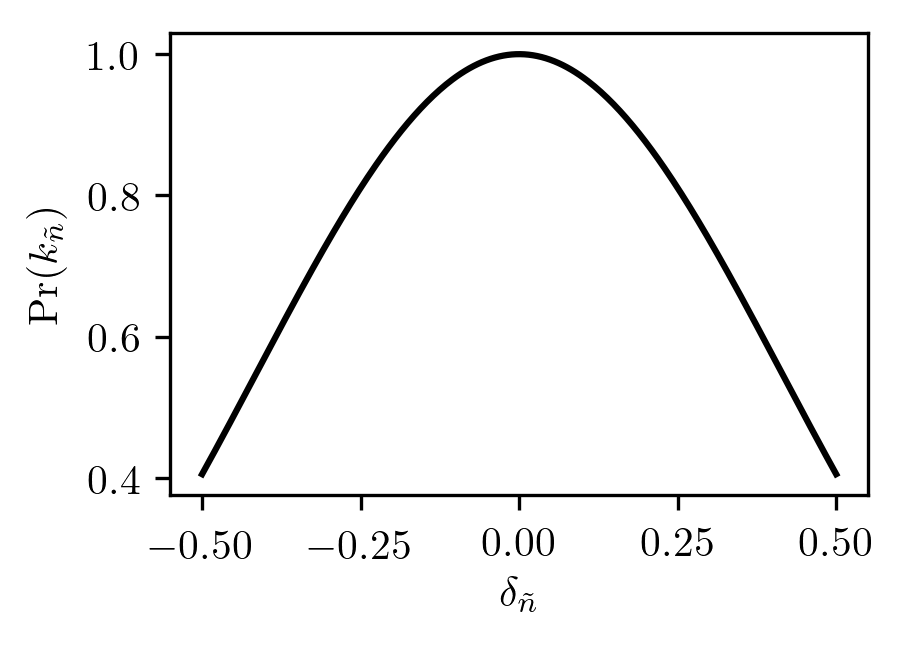It's similar for other $m$; the overall idea is that we are more likely to get the right answer when $| \delta_{\tilde{n}} |$ is smaller. Surprisingly, for large $| \delta_{\tilde{n}} |$, the probability can be quite low, even though we started with the system already in an eigenstate. As we'll see later, this isn't a cause for concern because this is just a consequence of adjacent bins sharing the probability.

If we don't suppose that we started from a single eigenstate, then there are several eigenvalues that could share the same $k_n$. Therefore a given $p$ could match more than one eigenstate and things get more complicated. Let's not go there just yet.

Wait, hold on, what's this about modular arithmetic?

Given an eigenvalue $\varepsilon$ of the Hamiltonian $\hat{H}_\mathrm{U}$, we can trivially find the corresponding eigenvalue $e^{2\pi i \varepsilon T / h}$ of $\hat{U}_\mathrm{U}^{2^m}$. However, because the complex logarithm is multivalued, the inverse procedure (to find the phase $\theta$ of $e^{2\pi i \theta}$) can only get us the fractional part: for any $\theta$ we pick to be our answer, every element of the set $\theta + \mathbb{Z}$ is also a valid answer. It's no surprise that this multivaluedness is an issue for us, since the algorithm in question is specifically for finding eigenvalues of unitary operators, and we're doing our best to apply it to Hermitian operators.

Suppose, for example, that $m = 4$ and $\Delta t = 0.07 \, h / \mathrm{eV} \approx 0.3 \, \mathrm{fs}$. Then $T / h = 1.12 / \mathrm{eV}.$ Here are some hypothetical eigenvalues $\varepsilon$ of $\hat{H}_\mathrm{U}$ with the corresponding values in the algorithm:

Naturally, we can only resolve 16 different outcomes in this example, and each one can represent infinitely many eigenvalues. Repeats in this table are marked with arcane symbols.

In general, measuring a particular value $p$ (assuming that we are lucky and the measurement reflects the desired state in the first place) implies that there is an eigenvalue within $\frac{h}{2 T}$ of $p \frac{h}{T} + s \frac{h}{\Delta t}$ for some integer $s$. This partitions the real numbers into a lattice of intervals of length $h / T$ indexed by $p$ and $s$. That is, every real number $x$ can be identified with the tuple $(s, p, \delta)$ and written as $x = p \frac{h}{T} + s \frac{h}{\Delta t} + \delta \frac{h}{T} = \frac{h}{\Delta t} \left( s + \frac{p + \delta}{2^m} \right),$ where $p$ is an $m$-bit integer, $s$ is any old integer, and $-\frac{1}{2} < \delta \le \frac{1}{2}$. Schematically, we can draw the real number line split into infinitely many intervals of length $h / \Delta t$: The point marked by the cross is at approximately $(2, 1, 1/4)$.

In this example, $\frac{h}{T} \approx 0.893 \, \mathrm{eV},$ so $p = 0$ could mean a band of values (of width $0.893 \, \mathrm{eV}$) around $0 \, \mathrm{eV}$, $\pm 14.3 \, \mathrm{eV}$, $\pm 28.6 \, \mathrm{eV}$, and so on. We could increase $\Delta t$ in order to shrink the size of each repeated segment or increase $m$ in order to grow the dynamic range within a repeated segment; both of these increase $T$ and give us a tighter band around each value.

Simulated result

With all that in mind, let's set up some simulations of the circuit. We'll try it in a couple of different ways to get a better sense of how this could work in practice.

Harmonic oscillators

To warm up, let's attempt a simple black box calculation, where we just write the circuit in terms of exact unitary matrices that do all the work for us. Consider a pair of coupled harmonic oscillators with the Hamiltonian $\hat{H} = \frac{1}{2} \left( \hat{p}_1^2 + \hat{q}_1^2 \right) + \frac{1}{2} \left( \hat{p}_2^2 + \hat{q}_2^2 \right) + k \hat{q}_1 \hat{q}_2.$ A bit of grunt work (with help from Appendix C of my MSc thesis) reveals that when $|k| \le 1$, the ground state energy of this Hamiltonian is given by $\frac{\sqrt{1+k} + \sqrt{1-k}}{2}.$ We'll set $k = 0.1$ so that the coupling is not too strong, and we'll be expecting an energy around $0.998746$.

In the tensor product basis of the individual oscillators, the matrix elements are $\begin{aligned} \langle n_1' \, n_2' | \hat{H} | n_1 \, n_2 \rangle &= \delta_{n_1' n_1} \delta_{n_2' n_2} (n_1 + n_2 + 1) \\ &\qquad + \frac{1}{10} \frac{1}{\sqrt{2}} (\delta_{n_1',n_1+1} \sqrt{n_1+1} + \delta_{n_1',n_1-1} \sqrt{n_1}) \\ &\qquad\qquad \otimes \frac{1}{\sqrt{2}} (\delta_{n_2',n_2+1} \sqrt{n_2+1} + \delta_{n_2',n_2-1} \sqrt{n_2}), \end{aligned}$ and we can use them to construct the Hamiltonian in a finite basis:

 1
 2
 3
 4
 5
 6
 7
 8
 9
10
11
12
13
14
15
16
17
18
19
20
21
22
23
24
25
26

julia> using LinearAlgebra
julia> eye(n) = Matrix{Float64}(I, n, n);
julia> q(n) = Symmetric(diagm(1 => sqrt.(1.0:(n-1))))/sqrt(2);
julia> function H(n)
         result = kron(diagm(0 => 0.0:(n-1)) + 0.5I, eye(n))
         result .+= kron(eye(n), diagm(0 => 0.0:(n-1)) + 0.5I)
         result .+= 0.1 * kron(q(n), q(n))
         result
       end;
julia> H(3)
9×9 Array{Float64,2}:
 1.0   0.0        0.0        0.0        0.05       0.0        0.0        0.0        0.0
 0.0   2.0        0.0        0.05       0.0        0.0707107  0.0        0.0        0.0
 0.0   0.0        3.0        0.0        0.0707107  0.0        0.0        0.0        0.0
 0.0   0.05       0.0        2.0        0.0        0.0        0.0        0.0707107  0.0
 0.05  0.0        0.0707107  0.0        3.0        0.0        0.0707107  0.0        0.1
 0.0   0.0707107  0.0        0.0        0.0        4.0        0.0        0.1        0.0
 0.0   0.0        0.0        0.0        0.0707107  0.0        3.0        0.0        0.0
 0.0   0.0        0.0        0.0707107  0.0        0.1        0.0        4.0        0.0
 0.0   0.0        0.0        0.0        0.1        0.0        0.0        0.0        5.0
julia> eigvals(H(3))[1]
0.9987460864290645
julia> eigvals(H(10))[1]
0.998746073110322
julia> eigvals(H(20))[1]
0.998746073110361

We only need about 10 basis functions per oscillator to get a good ground state energy, and as expected it's only slightly perturbed by the coupling.

Since we don't have any specific units of energy in mind, we'll set $h = 1$ and measure times in units of reciprocal energy. To get the ground state energy close to the middle of the $p = 1$ bin, we'll need to have $T \approx 1$.

The QFT is straightforward:

1
2
3
4
5
6
7
8

julia> outer(v) = v * v';
julia> qft(m) = exp.(2pi*im*outer(0:(2^m-1))/2^m)/sqrt(2^m);
julia> round.(qft(2); digits=3)
4×4 Array{Complex{Float64},2}:
 0.5+0.0im   0.5+0.0im   0.5+0.0im   0.5+0.0im
 0.5+0.0im   0.0+0.5im  -0.5+0.0im  -0.0-0.5im
 0.5+0.0im  -0.5+0.0im   0.5-0.0im  -0.5+0.0im
 0.5+0.0im  -0.0-0.5im  -0.5+0.0im   0.0+0.5im

The controlled unitary is nearly as straightforward:

1
2
3

julia> oneat(m, j) = (A = zeros(2^m); A[j] = 1; A);
julia> U(n, dt) = exp(2pi*im*H(n)*dt);
julia> CU(m, n, dt) = sum(kron(diagm(0 => oneat(m, j)), U(n, dt*(j-1))) for j in 1:2^m);

Note the extra factor of $2\pi$ because we've set $h = 1$, not $\hbar = 1$.

The easiest thing to do is to start from the exact ground state of the coupled harmonic oscillators:

 1
 2
 3
 4
 5
 6
 7
 8
 9
10
11
12
13
14
15
16
17
18
19
20
21
22
23
24
25

julia> using Qutilities
julia> function circuit(m, n, dt, v)
         state = kron(oneat(m, 1), v)
         state = kron(qft(m), eye(n^2)) * state
         state = CU(m, n, dt) * state
         state = kron(qft(m)', eye(n^2)) * state
         state
       end;
julia> probs(m, n, state) = real(diag(ptrace(state*state', (2^m, n^2), 2)));
julia> m = 3;
julia> n = 10;
julia> dt = 0.12;
julia> v = eigvecs(H(n))[:, 1];
julia> @time result = circuit(m, n, dt, v);
  0.267273 seconds (36.49 k allocations: 208.943 MiB, 52.51% gc time)
julia> probs(m, n, result)
8-element Array{Float64,1}:
 0.0019258161476215308 
 0.9945138775769432    
 0.00164707690823041   
 0.0005043909090011376 
 0.0003010558351650097 
 0.00026042359597120573
 0.00030923686002463913
 0.0005381221670408925 

To do the partial trace over the harmonic oscillators and obtain outcome probabilities for measuring the control register, I'm using the partial trace implementation from the Qutilities package. We've chosen to use 3 qubits for the time being, giving us 8 possible outputs. The probability is clustered around $p = 1$, which means that our estimate for the answer is

1
2

julia> 1/(2^m * dt)
1.0416666666666667

which is indeed less than

1
2

julia> 0.5/(2^m * dt)
0.5208333333333334

away from the correct answer. It's actually only

1
2

julia> 1/(2^m * dt) - eigvals(H(n))[1]
0.0429205935563447

away from the correct answer, which is why our probabilities were so sharp.

Consider instead

 1
 2
 3
 4
 5
 6
 7
 8
 9
10
11
12
13

julia> dt = 0.0625784688247742;
julia> @time result = circuit(m, n, dt, v);
  0.249420 seconds (36.47 k allocations: 207.874 MiB, 57.87% gc time)
julia> probs(m, n, result)
8-element Array{Float64,1}:
 0.41053347451699485 
 0.4105334745170109  
 0.050622325138180865
 0.02260097956518265 
 0.01624322077963387 
 0.016243220779633978
 0.022600979565182543
 0.05062232513818    

The only change was in the duration, so that the eigenvalue falls directly between the first two bins, and we do see that the bulk of the probability is split evenly between them. It's no coincidence that

1
2

julia> abs2((1-exp(2pi*im*0.5))/(1-exp(2pi*im*0.5/2^m)))/2^(2m)
0.41053347451700284

If we increase $m$ without changing $\Delta t$, we can better resolve the energy:

 1
 2
 3
 4
 5
 6
 7
 8
 9
10
11
12
13
14

julia> m = 6;
julia> n = 10;
julia> dt = 0.12;
julia> @time result = circuit(m, n, dt, v);
 35.094506 seconds (292.70 k allocations: 79.125 GiB, 10.46% gc time)
julia> probs(m, n, result)[6:12]
7-element Array{Float64,1}:
 0.010572912417752508
 0.026927549529518778
 0.1668693082196445  
 0.6899738964388513  
 0.042462317880069926
 0.013872943502266583
 0.006822244464881193

(This is two orders of magnitude slower.) We see that the majority of the probability is in bin 8, with a little bit in bin 7. This is reasonable, as the true energy is closer to

1
2

julia> 8/(2^m * dt)
1.0416666666666667

than to

1
2

julia> 7/(2^m * dt)
0.9114583333333334

Here's what the probability distribution looks like for a variety of $m$ values: Because we're keeping $\Delta t$ constant at $0.12$, the range of $\varepsilon$ doesn't change, but each bin gets smaller and the negative region shrinks.

We can also keep $m$ constant at $3$ and increase 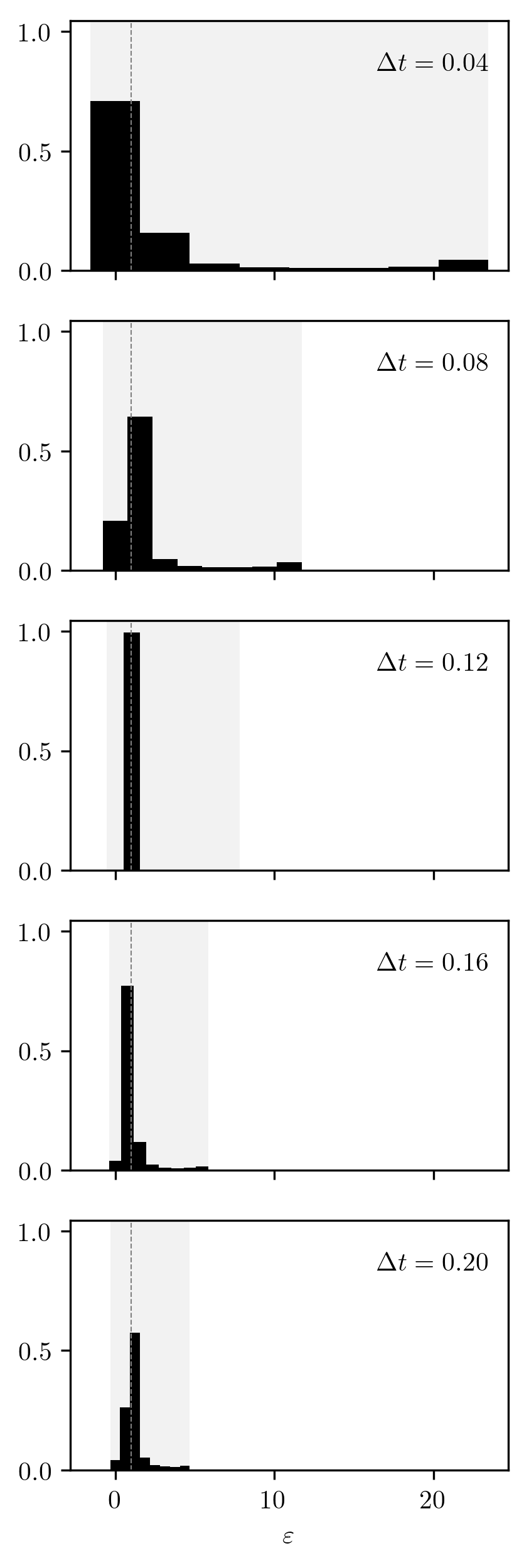$\Delta t$ (and $T$): The long and the short of it is that this seems to always work reasonably well, but it works best when the duration is tuned correctly.

The energy of the first excited state is

1
2
3
4

julia> eigvals(H(10))[2]
1.947429371160866
julia> eigvals(H(20))[2]
1.9474293711608688

We can also correctly predict it:

 1
 2
 3
 4
 5
 6
 7
 8
 9
10
11
12
13
14
15
16

julia> m = 3;
julia> n = 10;
julia> dt = 0.12;
julia> v = eigvecs(H(n))[:, 2];
julia> @time result = circuit(m, n, dt, v);
  0.124010 seconds (36.49 k allocations: 208.943 MiB, 3.94% gc time)
julia> probs(m, n, result)
8-element Array{Float64,1}:
 0.005527928092659891 
 0.02212701112663486  
 0.9460673221302545   
 0.013450918545547691 
 0.004501970310266165 
 0.0027946158277947124
 0.002487762931857694 
 0.0030424710349814745

Finally, here's an example (with $m = 5$ and $\Delta t = 0.16$) of the two eigenstates $| 0 \rangle$ and $| 2 \rangle$, as well as the superposition 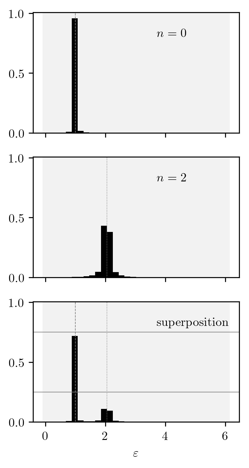$\frac{\sqrt{3} | 0 \rangle + | 2 \rangle}{2}:$ The horizontal lines are at $1/4$ and $3/4$. If we start with a superposition of eigenstates, we seem to obtain the weighted sum of the probability distributions.

This example highlights the fact that the SUT doesn't need to be expressed in terms of qubits: the input state $| \psi \rangle$ can in principle be whatever state you need it to be. Although the control register is expressed in the basis $\{ | 0 \rangle, | 1 \rangle \}^{\otimes m}$ of $m$ two-level systems, the remaining subsystem in this example is a genuine many-body quantum system. Of course, we must represent it by truncating its basis for practical reasons, but if we could implement a controlled unitary for this algorithm in the lab, there is no conceptual reason why it would need to act on a finite Hilbert space.

Transverse field Ising model

To appeal more to the spin-minded, we also look at the critical transverse field Ising model. The Hamiltonian for $L = 2$ spins is $\hat{H} = -\hat{\sigma}^z_1 \hat{\sigma}^z_2 - \hat{\sigma}^x_1 - \hat{\sigma}^x_2,$ and the formula $1 - \csc{\frac{\pi}{4L + 2}}$ gives us a ground state energy of $-2.236068$. Finally, a negative energy to really play with the modular wraparound!

Recall that $\begin{aligned} \hat{\sigma}^z | 0 \rangle &= | 0 \rangle \\ \hat{\sigma}^z | 1 \rangle &= -| 1 \rangle \end{aligned}$ and $\begin{aligned} \hat{\sigma}^x | 0 \rangle &= | 1 \rangle \\ \hat{\sigma}^x | 1 \rangle &= | 0 \rangle. \end{aligned}$ This means that (starting over in a fresh session) the Hamiltonian looks like

1
2
3
4
5
6
7
8

julia> H = -kron([1 0; 0 -1], [1 0; 0 -1]);
julia> H += -kron([0 1; 1 0], [1 0; 0 1]);
julia> H += -kron([1 0; 0 1], [0 1; 1 0])
4×4 Array{Int64,2}:
 -1  -1  -1   0
 -1   1   0  -1
 -1   0   1  -1
  0  -1  -1  -1

Because it's a bit circular to try to find an eigenvalue of a Hamiltonian by first exactly exponentiating it (which requires one to know all its eigenvalues), we will be more honest this time. We will also split the register-controlled unitary into several qubit-controlled unitaries for purposes of realism. The QFT is annoying to express in terms of more primitive gates, so we'll forgo that.

Since we're going to break the controlled unitary up into $m$ little pieces, we're going to need to evaluate $e^{2\pi i \hat{H} 2^j \Delta t}$ for $j = 0, \ldots, m-1$ (again having set $h = 1$ and using the appropriate units of time). To avoid diagonalizing $\hat{H}$, we will Trotterize the exponential: $e^{2\pi i \hat{H} 2^j \Delta t} \approx \left( e^{-2\pi i \hat{\sigma}^z_1 \hat{\sigma}^z_2 \tau} e^{-2\pi i \hat{\sigma}^x_1 \tau} e^{-2\pi i \hat{\sigma}^x_2 \tau} \right)^{P_j},$ where $2^j \Delta t = P_j \tau = 2^j P_0 \tau.$ Sadly, this gives us one more parameter to tweak, but this is a tolerable burden.

Speaking of parameters, if we pick $m = 3$ and $\Delta t = 0.17$, we should get the ground state somewhere close to the middle of bin 5. Specifically,

1
2
3
4

julia> m = 3;
julia> dt = 0.17;
julia> 5/(2^m * dt) - 1/dt
-2.205882352941176

which is off by only

1
2
3

julia> using LinearAlgebra
julia> 5/(2^m * dt) - 1/dt - eigvals(H)[1]
0.030185624558613622

compared to the bin width

1
2

julia> 1/(2^m * dt)
0.7352941176470588

Trivially, the matrix representation of $e^{-2\pi i \hat{\sigma}^z_1 \hat{\sigma}^z_2 \tau}$ is $\begin{pmatrix} e^{-2\pi i \tau} & 0 & 0 & 0 \\ 0 & e^{2\pi i \tau} & 0 & 0 \\ 0 & 0 & e^{2\pi i \tau} & 0 \\ 0 & 0 & 0 & e^{-2\pi i \tau} \end{pmatrix}.$ Nearly as trivially, the matrix representation of $e^{-2\pi i \hat{\sigma}^x \tau}$ is $\begin{pmatrix} \cos{(2\pi \tau)} & -i \sin{(2\pi \tau)} \\ -i \sin{(2\pi \tau)} & \cos{(2\pi \tau)} \end{pmatrix}.$

Now that we have all these pieces, we can code them up:

 1
 2
 3
 4
 5
 6
 7
 8
 9
10
11
12
13
14
15
16
17
18
19
20
21
22
23
24
25
26
27
28
29
30
31
32
33
34
35
36
37
38
39
40
41
42
43
44
45
46
47
48
49
50
51
52
53
54
55
56
57
58
59
60
61
62
63
64
65
66
67

julia> eye(n) = Matrix{Float64}(I, n, n);
julia> U_sigma_z(tau) = diagm(0 => exp.(2pi*im*[-1, 1, 1, -1]*tau));
julia> round.(U_sigma_z(0.25); digits=3)
4×4 Array{Complex{Float64},2}:
 0.0-1.0im  0.0+0.0im  0.0+0.0im  0.0+0.0im
 0.0+0.0im  0.0+1.0im  0.0+0.0im  0.0+0.0im
 0.0+0.0im  0.0+0.0im  0.0+1.0im  0.0+0.0im
 0.0+0.0im  0.0+0.0im  0.0+0.0im  0.0-1.0im
julia> U_sigma_x(tau) = [cos(2pi*tau) -im*sin(2pi*tau); -im*sin(2pi*tau) cos(2pi*tau)];
julia> round.(U_sigma_x(0.25); digits=3)
2×2 Array{Complex{Float64},2}:
 0.0+0.0im  0.0-1.0im
 0.0-1.0im  0.0+0.0im
julia> outer(v) = v * v';
julia> qft(m) = exp.(2pi*im*outer(0:(2^m-1))/2^m)/sqrt(2^m);
julia> oneat(m, j) = (A = zeros(2^m); A[j] = 1; A);
julia> function CU(m, j, tau)
         result = zeros(ComplexF64, 2^m*4, 2^m*4)
         for k in 1:2^m
           if (k-1) & (1<<(j-1)) == 0
             result .+= kron(diagm(0 => oneat(m, k)), eye(2), eye(2))
           else
             X = kron(diagm(0 => oneat(m, k)), U_sigma_z(tau))
             X *= kron(diagm(0 => oneat(m, k)), U_sigma_x(tau), eye(2))
             X *= kron(diagm(0 => oneat(m, k)), eye(2), U_sigma_x(tau))
             result .+= X
           end
         end
         result
       end;
julia> using Qutilities
julia> function circuit(m, dt, P0, v)
         state = kron(oneat(m, 1), v)
         state = kron(qft(m), eye(4)) * state
         for j in 1:m
           for _ in 1:(P0*2^(j-1))
             state = CU(m, j, dt/P0) * state
           end
         end
         state = kron(qft(m)', eye(4)) * state
         state
       end;
julia> probs(m, state) = real(diag(ptrace(state*state', (2^m, 4), 2)));
julia> v = eigvecs(H)[:, 1];
julia> for P0 in [1, 2, 5, 10, 100, 1000]
         println(P0)
         @time result = circuit(m, dt, P0, v);
         println(probs(m, result)[6])
       end;
1
  0.002621 seconds (1.86 k allocations: 2.976 MiB)
0.10734424166614077
2
  0.005387 seconds (3.70 k allocations: 5.908 MiB)
0.9075674144312382
5
  0.015230 seconds (9.20 k allocations: 14.703 MiB, 10.64% gc time)
0.9890106048450764
10
  0.027400 seconds (18.37 k allocations: 29.361 MiB, 5.04% gc time)
0.9934267922822306
100
  0.257648 seconds (183.43 k allocations: 293.210 MiB, 4.03% gc time)
0.9945435690246536
1000
  2.541286 seconds (1.83 M allocations: 2.863 GiB, 4.22% gc time)
0.9945539075921477

It appears that we get quite good results with just 10 Trotter factors, although we are able to improve the probabilities beyond that with rapidly diminishing results.

Despite the realism achieved in CU by having a separate controlled gate for each term of the Hamiltonian, I must admit that I've still cheated for all of the results, by choosing not only an appropriate duration, but also the exact ground state as the starting state. Trying random values for these quantities should still allow us to spot all four eigenvalues of this Hamiltonian. For reference, they are

1
2
3
4
5
6

julia> eigvals(H)
4-element Array{Float64,1}:
 -2.23606797749979  
 -0.9999999999999998
  1.0               
  2.2360679774997885

Here are some random attempts with 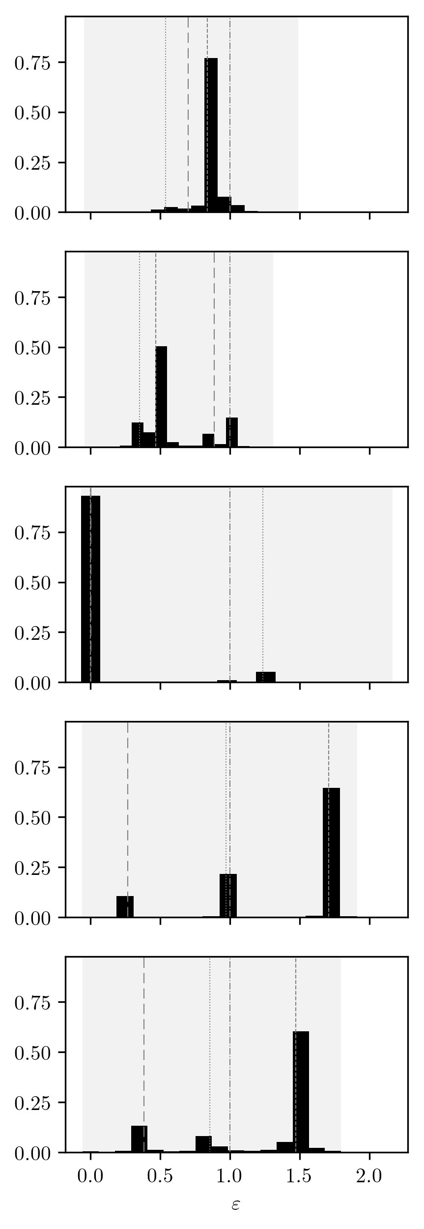$m = 4$ and $P_0 = 20$: The peaks are unpredictably distributed, but always in line with the eigenvalues! Note how the exact eigenvalues jump around between attempts because the varying total duration changes the energy range.

In conclusion, I think it's safe to claim that the algorithm works extremely well in practice for its intended usage (finding the eigenvalue of a known eigenvector of a unitary operator), but it can also be applied to extract some eigenvalue information out of a Hermitian operator.

Before we part ways, I want to show you one last example. The following plots show the change in the distribution as $\Delta t$ is gradually changed so that the target eigenvalue moves from the exact middle of a bin to the very edge of that bin: 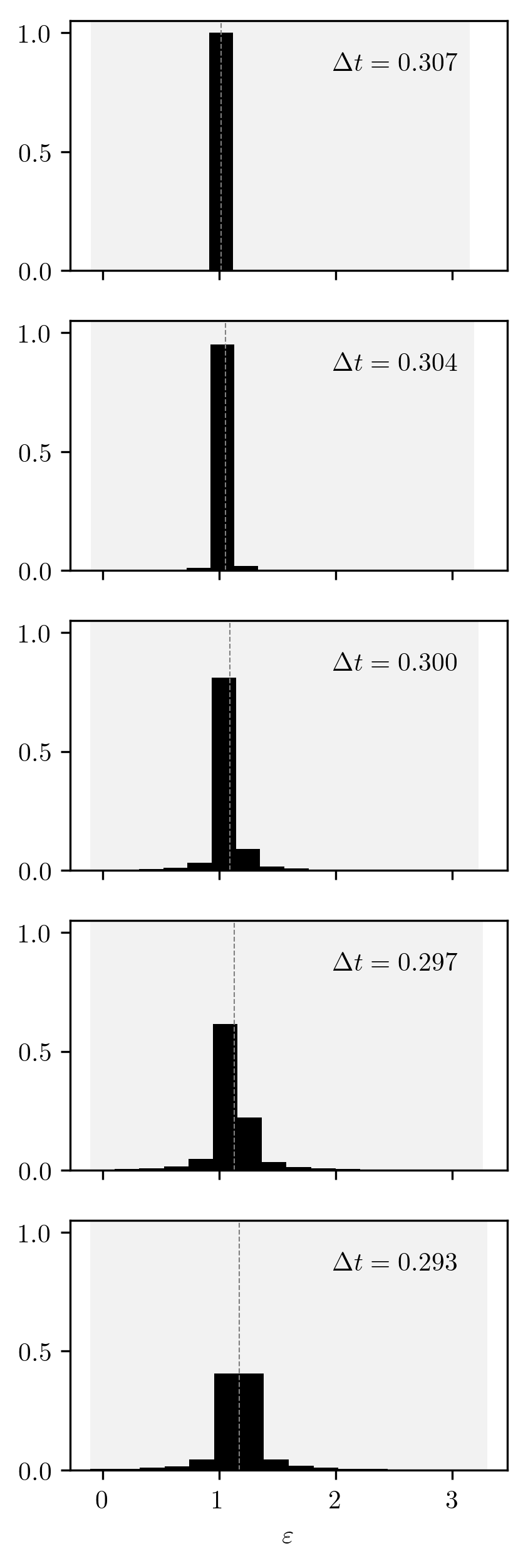The distribution gradually melts, but not all the way into a puddle.