Markov chain quasi-Monte Carlo
2020-01-30A 2005 paper by Owen and Tribble titled "A quasi-Monte Carlo Metropolis algorithm" (open access PDF) shows how to use the Metropolis–Hastings (MH) algorithm with proposal configurations generated using a quasi-random sequence. Unfortunately, the authors do not explicitly label any progression of steps as "the algorithm", so a bit of work is required to identify it.
If their algorithm is both practical and as effective as they claim, it should be extremely useful, since many real-world applications of Monte Carlo are Markov chain Monte Carlo (MCMC), and there's no obvious way to combine MCMC with quasi-Monte Carlo (QMC). Consider this quote from the paper:
Clear and even humorous failures will arise from using van der Corput points in MCMC. Morokoff and Caflisch describe an example where a heat particle supposed to undergo a symmetric random walk will instead move only to the left when sampled by van der Corput points.
On the other hand, they also mention this:
In the numerical examples we tried, our hybrid of QMC and MCMC always reduced the variance, sometimes by a factor of >200.
It seems that getting the hybridization right is non-trivial, but possibly worth it.
I'm first going to outline the algorithm from this paper as I understand it. Then, to verify my understanding, I'll try it out on a couple of examples.
Algorithm overview
As best as I can tell, the essence of the algorithm appears about half-way through the paper in Eqs. (4) and (5). Upon an initial skimming, it's easy to gloss over these equations, because they resemble the standard MH scheme: propose a random move, and conditionally accept it. However, the key here is that the points are not pseudo-random, but instead form a completely uniformly distributed (CUD) sequence. And not just any old CUD sequence, but specifically the output of a linear congruential generator (LCG) with a short period . The output values are then scaled by to make each one sit on the unit interval.
At each step of this algorithm, consecutive points are taken from the LCG; the last one is used to accept or reject, and the others are used for the proposal. Consider, for example, the LCG with modulus and the recurrence relation which has a period of : For , we get (arbitrarily starting the cycle at )
| Proposal | Accept | |
|---|---|---|
(The alternating cycles are alternatively bolded and not.) At this point, we have exhausted all possible combinations after running through the entire LCG times.
Suppose instead that . Then we seem to get
| Proposal | Accept | |
|---|---|---|
This is no good, because we've only obtained half of the possible combinations, but we've looped through them twice. Instead, we must introduce a skip in the sequence if we sense that we are repeating ourselves:
| Proposal | Accept | |
|---|---|---|
Much better. Although I can't reconcile this with Eqs. (4) and (5), which seem to have no provision for such an offset; perhaps this is explained elsewhere.
Here is an inefficient Julia function that takes an LCG with modulus N and generates d-tuples:
1 2 3 4 5 6 7 8 9 10 11 12 13 14 15 16 17 18 19 20 21 | function lcg_tuples(lcg::Function, N::Int, d::Int)
r = 1
seen = Set{Int}()
result = Vector{Int}[]
for _ in 1:(N-1)
while r in seen
r = lcg(r)
end
push!(seen, r)
tup = Array{Int}(undef, d)
for i in 1:d
tup[i] = r
r = lcg(r)
end
push!(result, tup)
end
result
end
|
For example,
1 2 3 4 5 6 7 8 9 10 11 12 13 14 15 16 17 | julia> lcg_tuples((r -> 3r%7), 7, 5)
6-element Array{Array{Int64,1},1}:
[1, 3, 2, 6, 4]
[5, 1, 3, 2, 6]
[4, 5, 1, 3, 2]
[6, 4, 5, 1, 3]
[2, 6, 4, 5, 1]
[3, 2, 6, 4, 5]
julia> lcg_tuples((r -> 3r%7), 7, 2)
6-element Array{Array{Int64,1},1}:
[1, 3]
[2, 6]
[4, 5]
[3, 2]
[6, 4]
[5, 1]
|
The easiest way to obtain all combinations is to slide a window of length through the LCG:
| Proposal | Accept | |
|---|---|---|
However, this produces overlapping tuples, while the algorithm is built around nonoverlapping ones. Still, we can write a function that produces this output:
1 2 3 4 5 6 7 8 9 10 11 12 13 14 15 16 17 18 19 | function lcg_tuples_overlap(lcg::Function, N::Int, d::Int)
r = 1
result = Vector{Int}[]
for _ in 1:(N-1)
tup = Array{Int}(undef, d)
tup[1] = r
r_next = r = lcg(r)
for i in 2:d
tup[i] = r
r = lcg(r)
end
push!(result, tup)
r = r_next
end
result
end
|
It gives us
1 2 3 4 5 6 7 8 | julia> lcg_tuples_overlap((r -> 3r%7), 7, 2)
6-element Array{Array{Int64,1},1}:
[1, 3]
[3, 2]
[2, 6]
[6, 4]
[4, 5]
[5, 1]
|
We'll see how this fails us later.
It is also important to introduce some randomization to the points in order to be able to estimate error bars for the computed value. The authors do this using Cranley–Patterson rotation, which shifts all the random values by a constant (pseudo-random) vector and then folds them back into the unit interval. For example:
1 2 3 4 5 6 7 8 9 10 | julia> tups = lcg_tuples((r -> 3r%7), 7, 5);
julia> v = [0.1, 0.2, 0.3, 0.4, 0.5];
julia> [round.((tup ./ 7 .+ v) .% 1; digits=3) for tup in tups]
6-element Array{Array{Float64,1},1}:
[0.243, 0.629, 0.586, 0.257, 0.071]
[0.814, 0.343, 0.729, 0.686, 0.357]
[0.671, 0.914, 0.443, 0.829, 0.786]
[0.957, 0.771, 0.014, 0.543, 0.929]
[0.386, 0.057, 0.871, 0.114, 0.643]
[0.529, 0.486, 0.157, 0.971, 0.214]
|
The algorithm therefore appears to be a modification of the standard MH algorithm. The differences are:
- Instead of a pseudo-random number generator (RNG), one uses an LCG and a pseudo-random vector . These are applied as described above, to produce shifted, nonoverlapping tuples of quasi-random numbers, which are fed into the proposal function and the acceptance decision step.
- Running through the entire Markov chain only generates a single estimate, and this process must be repeated several times with different vectors . The resulting values are combined to compute the mean and its standard error.
It is often convenient to use a nonhomogeneous proposal function. For example, when the different components of the state vector are updated one at a time, and not all at once; in this case, there are as many proposal distributions as there are components. Unfortunately, I don't understand the explanation in the paper relating to subchains. Based on their second example, I'm going to guess that all the random numbers that are needed for one loop over the components (that is, of them) should be obtained simultaneously.
Now for some examples to see if I got this right.
Example 1: Mean of the standard normal distribution
As our first problem, we'll take the first example from the paper. The goal is to compute the mean of the standard normal distribution which is of course zero. Their random walk sampler proposes shifting by a random step drawn from a normal distribution with standard deviation , and they go through steps. Each step is accepted or rejected with the standard Metropolis criterion, which in this case involves the quantity This requires two uniformly-distributed random numbers at each step: one to determine the size of the step and one to choose whether to accept it. To generate a normally-distributed random number from the former, we'll use the formula involving the inverse of the complementary error function to invert the normal cumulative distribution function .
Monte Carlo
First, we use the unmodified MH algorithm.
Here's an example of pairs of pseudo-random numbers, each between and :
 And this is what it looks like if we zoom in on the middle :
 Pretty typical, with clumps and gaps.
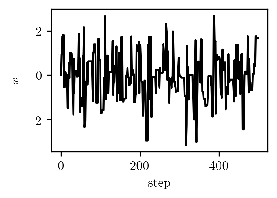
Using these points, we can generate a random walk starting at .
Here it is during the first steps:
 If we bin the locations after taking all the steps we get this histogram:
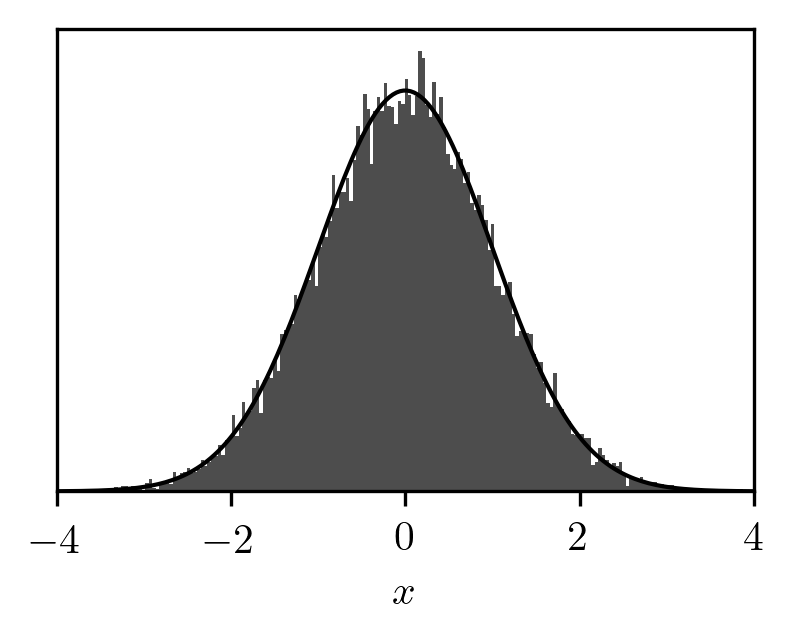
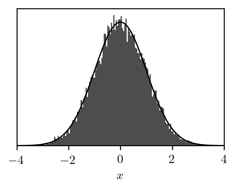 The exact result is in black, and we see that we're reasonably close to it.
If we use simultaneous walkers and average the results, here's what the overall instantaneous mean and standard error look like during the walks:
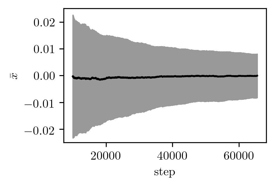 (Although in the paper the uncertainty is reported as the mean square error (MSE), it is represented here as the square root of the MSE.)
As the walks get longer, we stabilize on the correct result of zero and the uncertainty shrinks.
Here's the final result for the Monte Carlo random walk:
| Mean | MSE | |
|---|---|---|
| Owen and Tribble (2005) | ||
| Present work |
The mean differs from the one reported in the paper, but we expect some fluctuations. More importantly, the MSE is extremely close, so it looks like we've done the easy part successfully.
Quasi-Monte Carlo
Here, things get slightly more involved.
In order to generate a CUD sequence, the authors use the LCG with the recurrence relation
which has a period of .
This is what the values look like after being paired up:
 Much more regular!
Here's the middle :

If we go on a random walk using these pairs, we get one that looks rather similar to the pseudo-random one:
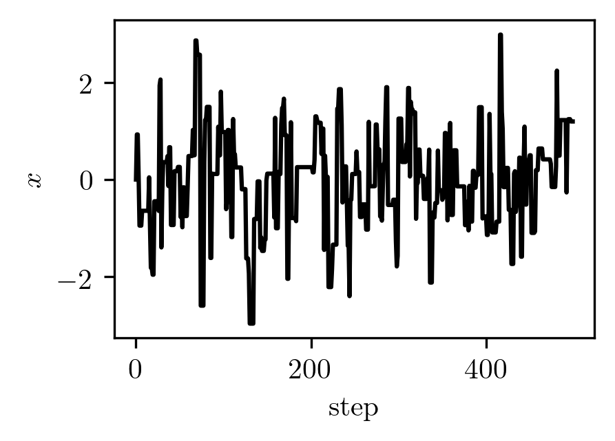 And the resulting histogram of positions doesn't look much improved:
 Yet the average over 300 realizations has smaller error bars than it did in the pseudo-random case:
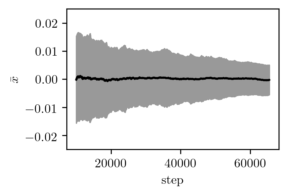 Despite having less estimated uncertainty, this looks a bit more rough than the pseudo-random case.
And this is the final result for the quasi-Monte Carlo random walk:
| Mean | MSE | |
|---|---|---|
| Owen and Tribble (2005) | ||
| Present work |
Again, our estimated error is close to that of Owen and Tribble, suggesting that we've reproduced their algorithm correctly. We have an MSE reduction compared to Monte Carlo of 2.41 which is very near their 2.65. For this example, it's really not apparent that the extra complexity is worth the reduction in error.
Quasi-Monte Carlo with overlapping tuples
I was curious about the importance of nonoverlapping tuples in this algorithm, so here are the results from the same quasi-Monte Carlo procedure as above, but with the pairs in a different order (one where the tuples overlap).
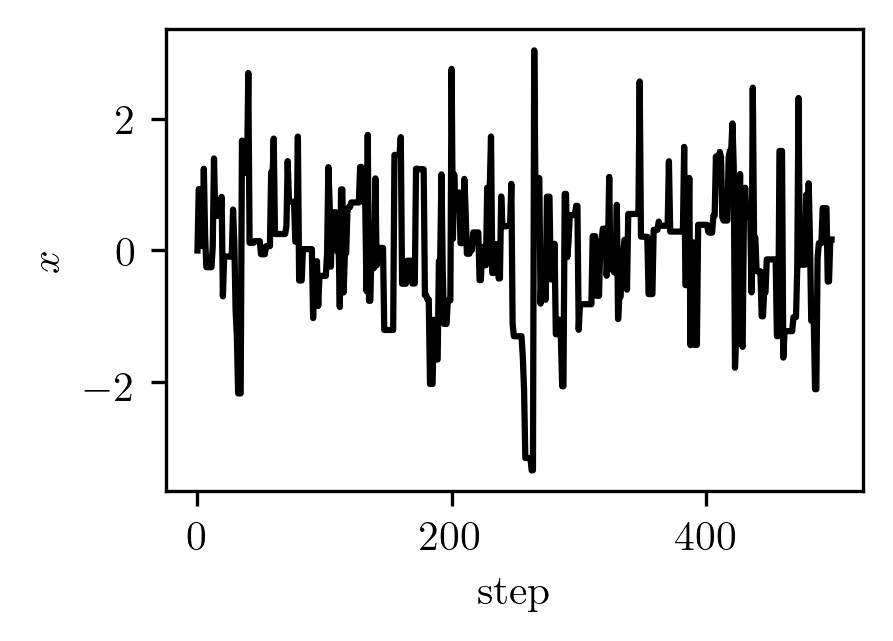
The random walk looks the same as always:
 However, the resulting distribution has a bit of lean to it:
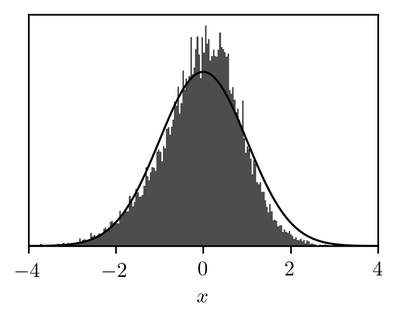 The mean seems to settle somewhere away from the correct value, and the estimate of the uncertainty does not decrease:
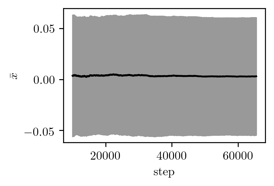
These results can't be trusted:
| Mean | MSE | |
|---|---|---|
| Present work |
Clearly, the ordering of the tuples implied by their nonoverlapping nature is crucial! Let's not do that again.
Example 2: Multivariate normal distribution
For the other example, we consider the integral
which evaluates to .
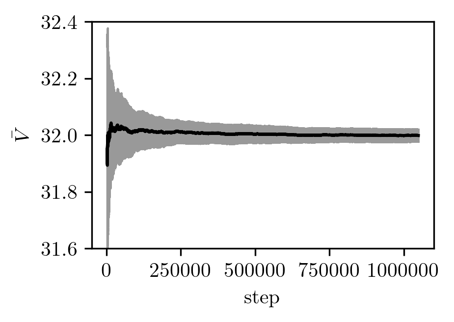
For the Monte Carlo updates, we take steps, and within each step we loop over the components of , requiring pseudo-random numbers to complete all the updates.
We propose to move each component by an amount drawn uniformly from , accepting according to the Metropolis criterion for the distribution
This process is repeated times, and the average of
from all these realizations is taken at each step.
The result looks acceptable:
In the quasi-Monte Carlo case, we use the LCG with the recurrence relation
where we've picked the parameters completely arbitrarily.
Here is the average over randomized walkers:
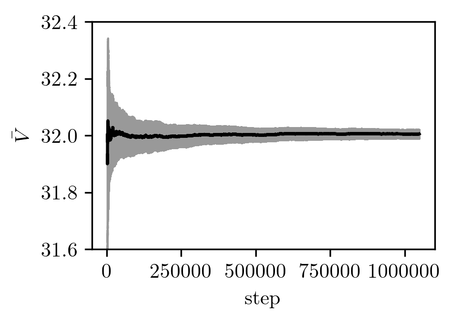
That this worked at all suggests that I may have understood the approach for nonhomogeneous proposal functions correctly! Additionally, we see a times reduction in the MSE:
| Mean | MSE | |
|---|---|---|
| Monte Carlo | ||
| Quasi-Monte Carlo |
Again, the hybrid method is not a clear slam dunk for this problem.
Conclusions
The algorithm as described above seems to be what Owen and Tribble had in mind. I was able to implement it and use it successfully for a pair of simple examples involving the normal distribution. In both cases, the improvements due to the hybrid method were present, but not nearly as impressive as the 200-fold reduction in variance that the authors saw in their second example (which I have not tried myself).
The article ends with the following:
We conclude by noting that the extra work in implementing MCMC with QMC is very small. One replaces the RNG by another RNG that has a smaller period and then uses the entire period one or more times.
However, it's not quite so simple:
- The RNG parameters must be chosen carefully for quasi-Monte Carlo. This is not an issue for Monte Carlo, since any modern pseudo-random number generator is typically treated as a black box.
- The entire sampling procedure must be repeated multiple times with randomization of the sampled points in order to estimate the standard error in quasi-Monte Carlo. In contrast, a single Monte Carlo random walk is often sufficient.
- The generation of nonoverlapping tuples is not particularly complex, but does need to be implemented.
With all this in mind, I think that there are certainly real applications that benefit from the hybrid method of Owen and Tribble, but some consideration is required before substituting it in place of MCMC for any specific application.